The Goal

SDF shapes are a flexible way to create resolution independent materials for UI and VFX. Resolving those SDFs into solid shapes can be tricky though, since you often run into aliasing and inconsistent edge treatment at different scales.

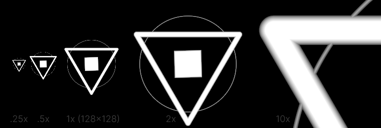
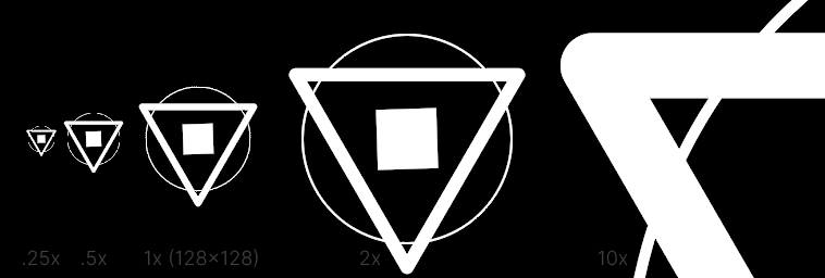
The objective is to turn some SDF gradient like this…

…into a black and white crisply-edged shape like this:

• Crisp anti-aliased edges regardless of scale.
• No artifacts or disintegration even with small edge widths.
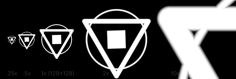
• Accurate designer-friendly measurements – in this example the Circle has a stroke width of 1px at 1x.

This is the ideal result we’re going for, and this doc will cover other methods and how to get there.

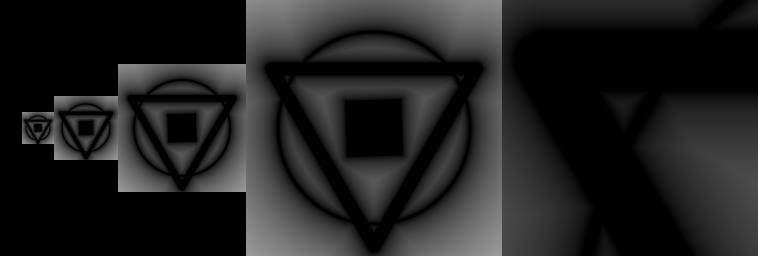
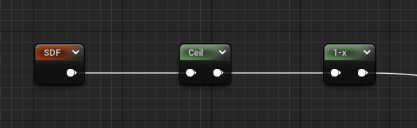
No Filter

The most basic method is to simply ceiling the value. Anything > 0 will be white and everything else black.

• The obvious result is a lot of aliasing, and the shapes can disappear at small scales.
• At 1x, you can notice the circle is designed to be exactly 1px, which we want to try to preserve in the next steps.
• A 1-x is used since SDFs natively have positive values on the outside, but we want white on the interior.

Smoothstep Fixed

A very common method of softening the edge is to use smoothstep.

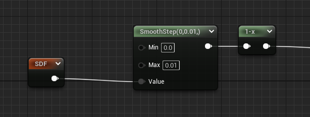
• Given a small-ranged Min and Max value, a smooth gradient is created which softens the shape nicely at 1x.
• Since the range is fixed right now, the shape is blurry at large scales and still aliased/disappearing when small.
• The circle at 1x appears larger than 1 pixel in width.
• This method is actually great when you’re going for a glow or shadow instead of crisp edges.

The magic number 0.01 is just a small-enough value such that the image looks crisp at 1x. Since the actual distance values of the SDF in this example are based on the default UVs (0..1), you can think of the gradient over which anti-aliasing occurs to have a width thats 1/100th the size of the image.

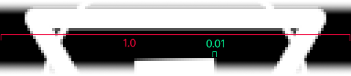
The large gradient seen in the 10x example then makes sense because that image size is 1280 (10 x 128), and 1280 x 0.01 is 12.8, giving a roughly 13 pixel edge. This may seem obvious or irrelevant but it helps when trying to understand the later examples.

Divide Fixed

Since we’re going for crisp edges, the smoothness of smoothstep is unnecessary and a divide can be used instead.

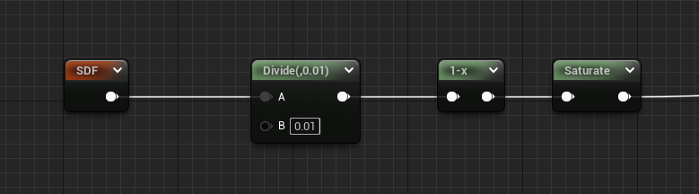
• At 10x you can notice the slightly harder linear gradient, but at 1x the difference is indistinguishable.
• Circle stroke width is still too large.
• A saturate is used to clamp the results to 0..1.

Divide Fixed Inner

The previous two methods naturally inflate the shape, since the shape itself has a boundary at 0, and the resulting edge gradients were between 0 and 0.01. To fix this, we can flip the SDF (multiply by -1), which will essentially perform the smoothing on the interior of each shape.

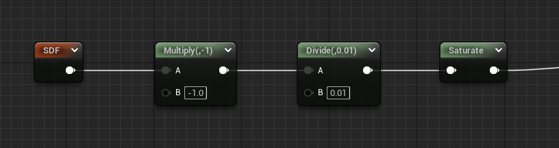
• The result is noticeably thinner at 10x since the ~13px gradient now goes inwards instead of out.
• The circle at 1x is looking a lot more like 1px wide, with some ok-not-great smoothing compared to ceiling.
• Ditched the 1-x operation from previous methods since the interior distances are now positive.

Filter Width

To finally solve the large gradient at 10x, we can use derivatives to determine the scale at which the material is viewed, and adjust accordingly. Using DDX and DDY, we calculate the change between neighboring pixels, which can be used directly in the divide. The calculated value is sometimes referred to as the filter width, a probably-more-apt name than the previously mentioned ‘smooth edge gradient width’.

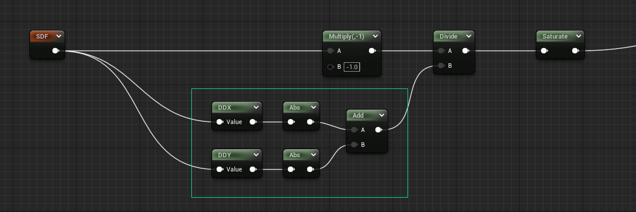
• The edge sharpness is now consistent regardless of scale.
• Basically perfect at 10x, but disintegrating at small scales, and even partially at 1x.

We use both the DDX and DDY (derivatives of X and Y), take their absolute values, and add them together. Which in this case will give slightly larger (and therefore smoother) values on diagonals, where both X and Y values of the SDF are changing.

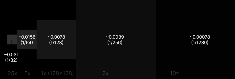
Visualizing SDF Derivatives

With this method we’re calculating what range we need to use to have a 1-pixel-wide edge gradient at all scales. With the example of a 128x128 image, if you picture a linear gradient going from 0..1 (like a default tex coord) the change from one pixel to the next would be 1/128 or 0.0078 (not dissimilar from our previous fixed value of 0.01). In this context it helps to think of the derivatives as the slope of the gradient. At smaller scales the slope is much larger, since from pixel to pixel the value changes quickly. At large scales the slope is much smaller.

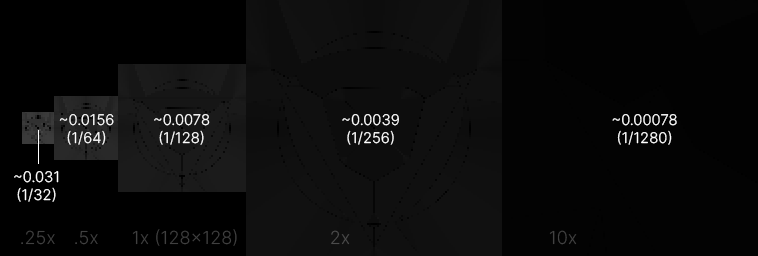
You may notice some artifacts in this image, which will have an impact later.

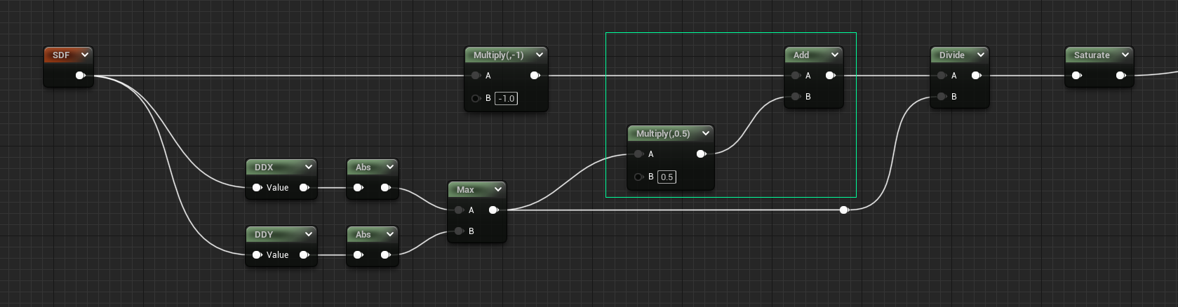
Filter Width Bias

Now that we’ve calculated the filter width, we can fix the biggest issue remaining, which is thin shapes dissolving into nothing. By adding the calculated filter width to the SDF first, we essentially inflate the shape again, but this time with a more intelligent value.

• The smaller line widths are now much more visible and stable, but still have some disintegration.
• The 1x circle looks pretty close to an expected 1px stroke as seen in other apps, even if it’s actually more like 2px in most places when you consider anti-aliasing.
• 10x still looks great, the small inflation of ~0.00078 does basically nothing.
• There’s still a few artifacts overall – at the top of the 1x circle, and in various intersections.

The reasoning for this method is: if we want to have a consistent edge treatment we need at least a minimum amount of visible shape over which to perform the filtering. So adding an inflation that’s in this case 50% of the filter width gives us content to display instead of shapes disappearing.

That magic value of 0.5 is intended such that half of the filter width is added to each ‘side’, so the total is 1x the filter width for strokes and small objects (e.g. when you consider the two sides of a stroke). If we added the full value of 1 the inflation becomes too noticeable and our 1px circle no longer looks like 1px. Try playing with this value to see how it affects the thinner lines.

We’ve also switched to using Max instead of Add for the filter width calculation, since the extra inflation of their combined values adds a bit too much softening.

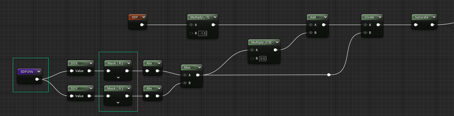
UV Filter Width Bias

If you compare the areas that are still problematic with the DDX visualization from before, you can see there are black spots where the derivatives just fail to calculate clean values. What’s nice about SDFs though, is that when calculated correctly their overall gradient will match that of the input UVs. So to achieve our original goal we can calculate the filter width on the UVs instead of the SDF.

• Beautiful, no notes… well… some notes:
• The overall image quality feels good but not better than many vector drawing applications.
• The .25x feels a tiny bit fuzzy, but it’s better than it disappearing when crunched to small sizes.
• The remaining artifacts and disintegration are gone.
• For the price, this seems more than acceptable.

Now that we’re giving DDX/DDY a float2, it will return a float2, and interestingly DDX will only output to R channel, and DDY to G channel. So we need to use component masks to grab the values this time.

The reason this method works better than the previous example is because the filter width calculation is much simpler for UVs. Since the ‘slope’ of undistorted UVs doesn’t change much, you get a reliable filter width across the whole image.

The other benefit of this method is that you can calculate the filter width for a set of UVs once, then reuse it for all SDF shapes generated from them. If you scale or distort the UVs though, you’ll need to calculate a new filter width. This method also may not work if you just don’t have access to the original SDF UVs, e.g. the SDF was generated by another tool or is coming from a texture. Even so, is there a way to recreate an approximation of them that’s good enough to serve this purpose?

More on DDX and DDY

It’s understandable that using the DDX/DDY of the SDF instead of the UVs causes more artifacts since the slope of an SDF changes, especially around the areas we want to sharpen, but it’s also likely due to how they are calculated. This article does a great job explaining. Some key pieces are copied here:

Internally, GPUs never run one instance of a pixel shader at a time. At the finest level of granularity, they are always running 32-64 pixels at the same time using a SIMD architecture. Within this, the pixels are further organized into 2x2 quads, so each group of 4 consecutive pixels in the SIMD vector corresponds to a 2x2 block of pixels on screen.

Derivatives are calculated by taking differences between the pixels in a quad. For instance, ddx will subtract the values in the pixels on the left side of the quad from the values on the right side, and ddy will subtract the bottom pixels from the top ones. The differences can then be returned as the derivative to all four pixels in the quad.

This is a big reason why I prefer using the DDX of the UVs, since comparing quads is much more stable.

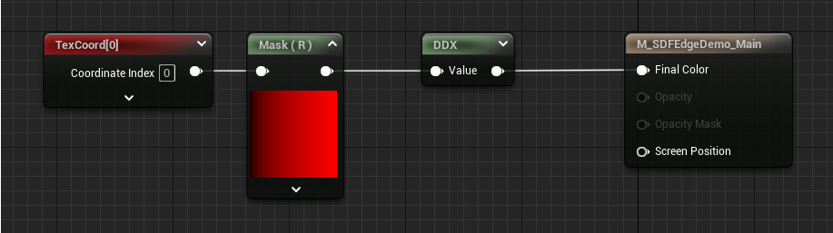
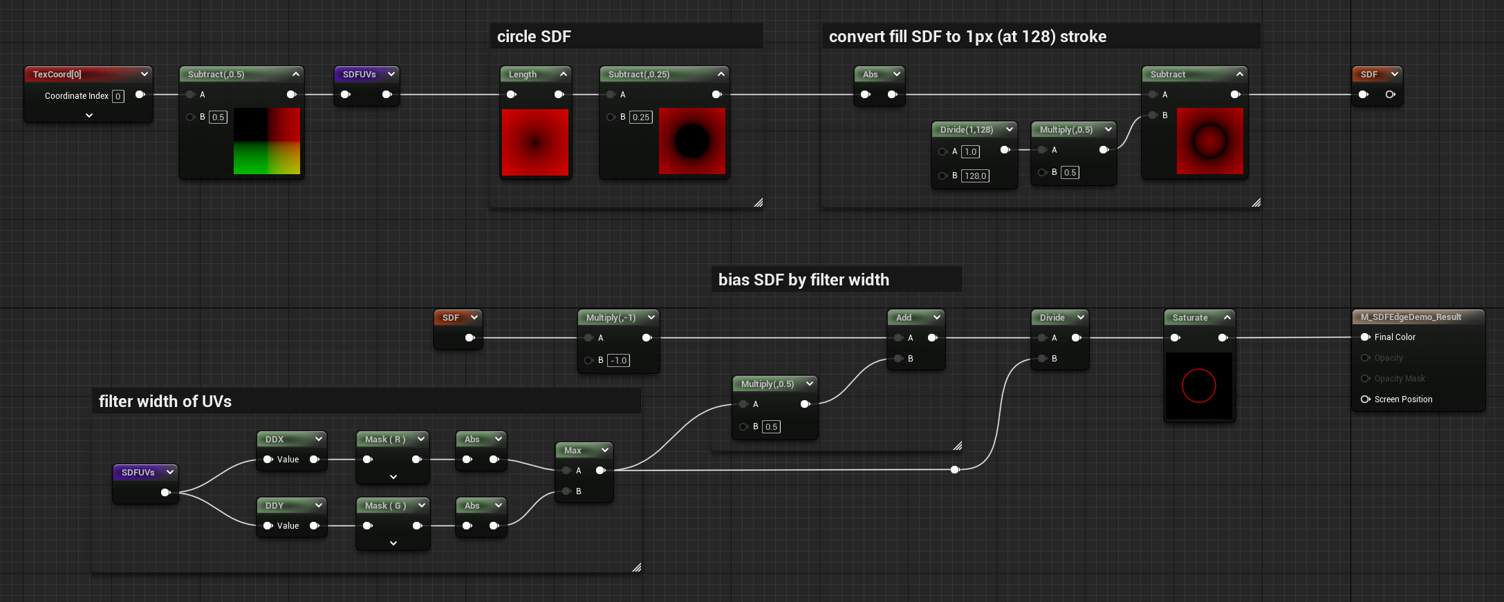
Full Example

Here’s a full material graph of a Circle SDF, converted to a stroke, then filled using the last technique above, with some nodes expanded to see previews.

To make this more versatile you can use material functions for the main operations of this graph, and get something like the following:

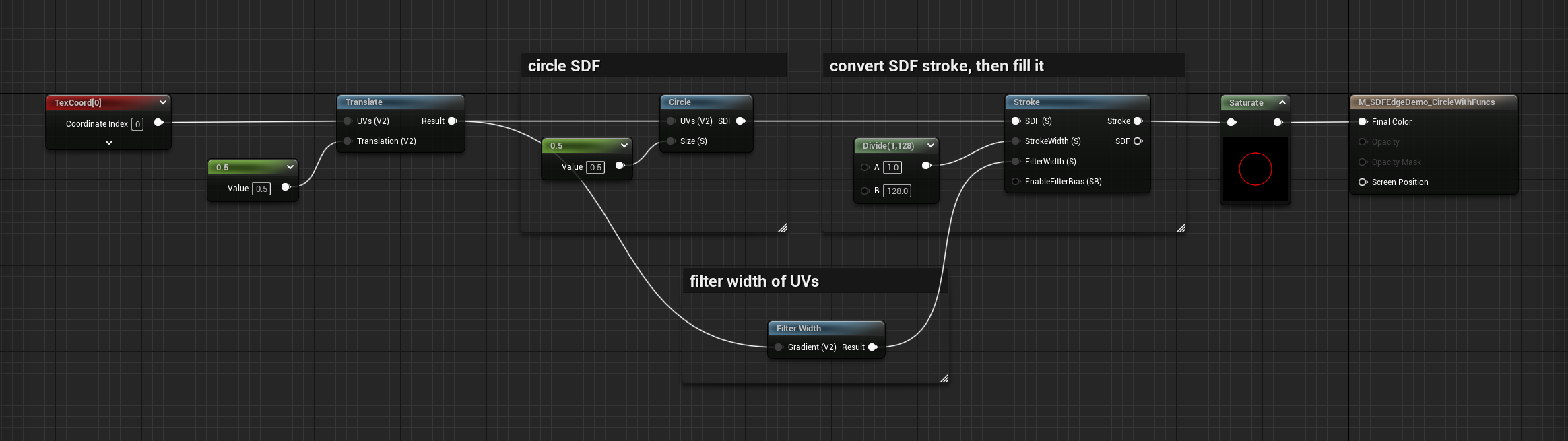
These functions are available in the MGFX plugin so check them out!

Performance

Here’s some performance info according to the material editor stats for each method, taken using a single solid circle SDF:

• Circle SDF raw: 27 instructions
• Ceiling: 29 instructions
• Smoothstep Fixed: 31 instructions
• Divide Fixed: 28 instructions
• Divide Fixed Inner: 28 instructions
• Filter Width: 31 instructions
• Filter Width Bias: 32 instructions
• UV Filter Width Bias: 32 instructions

People say not to take these stats at face value, since in practice the results can vary. But the bias obviously adds an additional instruction, so in the material functions of MGFX plugin it’s actually an optional feature you can enable via static bool depending on whether the shape needs it (notice the unconnected EnableFilterBias input of the last example graph). Large shapes and fat lines would likely never need the bias since they won’t disappear at small scales.

More great SDF articles you should read:

• 2D SDF - Basic Shapes and Visualization by Fabrizio Bergamo
• What Are SDFs Anyway? by Joyrok